Unsupervised Learning (Clustering)
Segment mall customers into meaningful groups for targeted marketing strategies.
Mall_Customers.csv (https://www.kaggle.com/datasets/vjchoudhary7/customer-segmentation-tutorial-in-python/data)CustomerID, Gender,
Age, Annual Income (k$),
Spending Score (1-100)import numpy as np
import pandas as pd
import matplotlib.pyplot as plt
import seaborn as sns
from sklearn.preprocessing import StandardScaler
from sklearn.cluster import KMeans, AgglomerativeClustering
from sklearn.metrics import silhouette_score
from scipy.cluster.hierarchy import linkage, fclusterdata = pd.read_csv("Mall_Customers.csv")data.head()| CustomerID | Gender | Age | Annual Income (k$) | Spending Score (1-100) | |
|---|---|---|---|---|---|
| 0 | 1 | Male | 19 | 15 | 39 |
| 1 | 2 | Male | 21 | 15 | 81 |
| 2 | 3 | Female | 20 | 16 | 6 |
| 3 | 4 | Female | 23 | 16 | 77 |
| 4 | 5 | Female | 31 | 17 | 40 |
data.shape(200, 5)
clean_data = data.copy()
clean_data.columns = clean_data.columns.str.strip()clean_data.isnull().sum()CustomerID 0
Gender 0
Age 0
Annual Income (k$) 0
Spending Score (1-100) 0
dtype: int64
duplicate_count = int(clean_data.duplicated().sum())
print("Duplicate rows:", duplicate_count)Duplicate rows: 0
clean_data = clean_data.drop_duplicates().reset_index(drop=True)
print("Shape after cleaning:", clean_data.shape)Shape after cleaning: (200, 5)
clean_data.describe()| CustomerID | Age | Annual Income (k$) | Spending Score (1-100) | |
|---|---|---|---|---|
| count | 200.000000 | 200.000000 | 200.000000 | 200.000000 |
| mean | 100.500000 | 38.850000 | 60.560000 | 50.200000 |
| std | 57.879185 | 13.969007 | 26.264721 | 25.823522 |
| min | 1.000000 | 18.000000 | 15.000000 | 1.000000 |
| 25% | 50.750000 | 28.750000 | 41.500000 | 34.750000 |
| 50% | 100.500000 | 36.000000 | 61.500000 | 50.000000 |
| 75% | 150.250000 | 49.000000 | 78.000000 | 73.000000 |
| max | 200.000000 | 70.000000 | 137.000000 | 99.000000 |
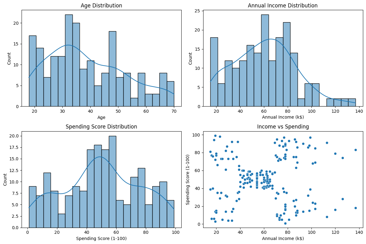
fig, axes = plt.subplots(2, 2, figsize=(12, 8))
sns.histplot(clean_data["Age"], bins=20, kde=True, ax=axes[0, 0])
axes[0, 0].set_title("Age Distribution")
sns.histplot(clean_data["Annual Income (k$)"], bins=20, kde=True, ax=axes[0, 1])
axes[0, 1].set_title("Annual Income Distribution")
sns.histplot(clean_data["Spending Score (1-100)"], bins=20, kde=True, ax=axes[1, 0])
axes[1, 0].set_title("Spending Score Distribution")
sns.scatterplot(data=clean_data, x="Annual Income (k$)", y="Spending Score (1-100)", ax=axes[1, 1])
axes[1, 1].set_title("Income vs Spending")
plt.tight_layout()
plt.show()
feature_columns = ["Annual Income (k$)", "Spending Score (1-100)"]
X = clean_data[feature_columns].copy()X.head()| Annual Income (k$) | Spending Score (1-100) | |
|---|---|---|
| 0 | 15 | 39 |
| 1 | 15 | 81 |
| 2 | 16 | 6 |
| 3 | 16 | 77 |
| 4 | 17 | 40 |
scaler = StandardScaler()
X_scaled = scaler.fit_transform(X)X_scaled.shape(200, 2)
k_values = list(range(2, 11))
kmeans_scores = []
agg_scores = []
kmeans_inertia = []
for k in k_values:
kmeans_model_temp = KMeans(n_clusters=k, random_state=42, n_init=10)
kmeans_labels_temp = kmeans_model_temp.fit_predict(X_scaled)
agg_labels_temp = AgglomerativeClustering(n_clusters=k).fit_predict(X_scaled)
kmeans_scores.append(silhouette_score(X_scaled, kmeans_labels_temp))
agg_scores.append(silhouette_score(X_scaled, agg_labels_temp))
kmeans_inertia.append(kmeans_model_temp.inertia_)
best_k_kmeans = k_values[int(np.argmax(kmeans_scores))]
best_k_agg = k_values[int(np.argmax(agg_scores))]
print(f"Best k for K-Means: {best_k_kmeans} with silhouette score {max(kmeans_scores):.4f}")Best k for K-Means: 5 with silhouette score 0.5547
plt.figure(figsize=(6, 4))
plt.plot(k_values, kmeans_inertia, marker="o")
plt.title("K-Means Elbow Method")
plt.xlabel("k")
plt.ylabel("Inertia")
plt.show()
plt.figure(figsize=(6, 4))
plt.plot(k_values, kmeans_scores, marker="o", label="KMeans")
plt.plot(k_values, agg_scores, marker="o", label="Agglomerative")
plt.title("Silhouette Score vs k")
plt.xlabel("k")
plt.ylabel("Silhouette Score")
plt.legend()
plt.show()
score_table = pd.DataFrame({
"k": k_values,
"KMeans Silhouette": kmeans_scores,
"Agglomerative Silhouette": agg_scores
})
score_table| k | KMeans Silhouette | Agglomerative Silhouette | |
|---|---|---|---|
| 0 | 2 | 0.321271 | 0.384234 |
| 1 | 3 | 0.466585 | 0.461048 |
| 2 | 4 | 0.493907 | 0.492551 |
| 3 | 5 | 0.554657 | 0.553809 |
| 4 | 6 | 0.539880 | 0.538676 |
| 5 | 7 | 0.528149 | 0.519795 |
| 6 | 8 | 0.455215 | 0.430862 |
| 7 | 9 | 0.457085 | 0.437690 |
| 8 | 10 | 0.443171 | 0.433901 |
print("Best k for KMeans:", best_k_kmeans)
print("Best k for Agglomerative:", best_k_agg)Best k for KMeans: 5
Best k for Agglomerative: 5
hier_k_values = list(range(2, 11))
hier_scores = []
hier_labels_list = []
hier_linkage_matrix = linkage(X_scaled, method="ward")for k in hier_k_values:
labels = fcluster(hier_linkage_matrix, t=k, criterion="maxclust") - 1
hier_labels_list.append(labels)
hier_scores.append(silhouette_score(X_scaled, labels))
best_hier_index = int(np.argmax(hier_scores))
best_hier_k = hier_k_values[best_hier_index]
best_hier_score = hier_scores[best_hier_index]
hierarchical_labels = hier_labels_list[best_hier_index]hier_table = pd.DataFrame({
"k": hier_k_values,
"silhouette": hier_scores
})
hier_table| k | silhouette | |
|---|---|---|
| 0 | 2 | 0.384234 |
| 1 | 3 | 0.461048 |
| 2 | 4 | 0.492551 |
| 3 | 5 | 0.553809 |
| 4 | 6 | 0.538676 |
| 5 | 7 | 0.519795 |
| 6 | 8 | 0.430862 |
| 7 | 9 | 0.437690 |
| 8 | 10 | 0.433901 |
print("Best Hierarchical k:", best_hier_k)
print("Best Hierarchical silhouette:", best_hier_score)Best Hierarchical k: 5
Best Hierarchical silhouette: 0.5538089226688662
kmeans_model = KMeans(n_clusters=best_k_kmeans, random_state=42, n_init=10)
kmeans_labels = kmeans_model.fit_predict(X_scaled)
agg_model = AgglomerativeClustering(n_clusters=best_k_agg)
agg_labels = agg_model.fit_predict(X_scaled)
kmeans_score = silhouette_score(X_scaled, kmeans_labels)
agg_score = silhouette_score(X_scaled, agg_labels)
hier_score = best_hier_score
comparison = pd.DataFrame({
"Algorithm": ["KMeans", "Agglomerative", "Hierarchical"],
"Parameter (K)": [best_k_kmeans, best_k_agg, best_hier_k],
"Silhouette Score": [kmeans_score, agg_score, hier_score]
})
best_algorithm = comparison.loc[comparison["Silhouette Score"].idxmax(), "Algorithm"]
print(comparison)
print("Best algorithm:", best_algorithm) Algorithm Parameter (K) Silhouette Score
0 KMeans 5 0.554657
1 Agglomerative 5 0.553809
2 Hierarchical 5 0.553809
Best algorithm: KMeans
valid_comparison = comparison.dropna(subset=["Silhouette Score"]).reset_index(drop=True)
if len(valid_comparison) > 0:
best_algorithm = valid_comparison.loc[valid_comparison["Silhouette Score"].idxmax(), "Algorithm"]
else:
best_algorithm = "KMeans"
best_algorithm'KMeans'
clustered = clean_data.copy()
clustered["KMeans"] = kmeans_labels
clustered["Agglomerative"] = agg_labels
clustered["Hierarchical"] = hierarchical_labels
fig, axes = plt.subplots(1, 3, figsize=(18, 5))
for ax, column, title in zip(
axes,
["KMeans", "Agglomerative", "Hierarchical"],
["K-Means Clusters", "Agglomerative Clusters", "Hierarchical Clusters"],
):
sns.scatterplot(
data=clustered,
x="Annual Income (k$)",
y="Spending Score (1-100)",
hue=column,
palette="tab10",
ax=ax,
s=55,
)
ax.set_title(title)
ax.legend(title=column, bbox_to_anchor=(1.02, 1), loc="upper left")
plt.tight_layout()
plt.show()
if best_algorithm == "KMeans":
final_labels = kmeans_labels
elif best_algorithm == "Agglomerative":
final_labels = agg_labels
else:
final_labels = hierarchical_labels
clustered["BestCluster"] = final_labelsclustered[["Annual Income (k$)", "Spending Score (1-100)", "BestCluster"]]| Annual Income (k$) | Spending Score (1-100) | BestCluster | |
|---|---|---|---|
| 0 | 15 | 39 | 4 |
| 1 | 15 | 81 | 2 |
| 2 | 16 | 6 | 4 |
| 3 | 16 | 77 | 2 |
| 4 | 17 | 40 | 4 |
| ... | ... | ... | ... |
| 195 | 120 | 79 | 1 |
| 196 | 126 | 28 | 3 |
| 197 | 126 | 74 | 1 |
| 198 | 137 | 18 | 3 |
| 199 | 137 | 83 | 1 |
200 rows × 3 columns
cluster_summary = clustered.groupby("BestCluster")[["Age", "Annual Income (k$)", "Spending Score (1-100)"]].mean().round(2)
cluster_summary| Age | Annual Income (k$) | Spending Score (1-100) | |
|---|---|---|---|
| BestCluster | |||
| 0 | 42.72 | 55.30 | 49.52 |
| 1 | 32.69 | 86.54 | 82.13 |
| 2 | 25.27 | 25.73 | 79.36 |
| 3 | 41.11 | 88.20 | 17.11 |
| 4 | 45.22 | 26.30 | 20.91 |
cluster_counts = clustered["BestCluster"].value_counts().sort_index()
cluster_countsBestCluster
0 81
1 39
2 22
3 35
4 23
Name: count, dtype: int64
print("Final Decision")
print("Best Algorithm:", best_algorithm)Final Decision
Best Algorithm: KMeans
Reasons:
This mini project follows the full required flow: cleaning, visualization, preprocessing, model training, evaluation, best model selection, and learning conclusion.